Beamforming in Nullspace

Dear Nullspace Team,

I am currently working on an Integrated Sensing and Communication (ISAC) model using an 8x8 planar antenna array with polarization diversity employing wideband half-wavelength dipoles (tilted ±45º). Each antenna element consists of two crossed dipoles, where only one is active at a time. Below I attached a portion of my .jou file showing the creation of a single antenna element:

create surface rectangle width {w} height {L} zplane
#{a1 = Id("surface")}
split surface {a1} across location position {-w} 0 0 location position {w} 0 0
#{a1a = Id("surface")-1}
#{a1b = Id("surface")}

create surface rectangle width {L} height {w} zplane
#{a2 = Id("surface")}
split surface {a2} across location position 0 {-w} 0 location position 0 {w} 0
#{a2a = Id("surface")-1}
#{a2b = Id("surface")}

rotate surface {a1a} {a1b} {a2a} {a2b} angle 45 about Z
move surface {a1a} {a1b} {a2a} {a2b} x {0} y {0}

block 1 surface {a1a} {a1b}
block 2 surface {a2a} {a2b}
nsem assign surface {a1a} {a1b} {a2a} {a2b} material "PEC"
nsem voltage source "p1" pos surface {a1a} neg surface {a1b} impedance 50
nsem lumped load "l2" surface {a2a} {a2b} impedance 50 0

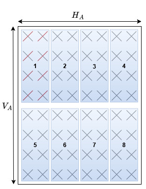
For beamforming, I am aggregating these dipoles into eight 4x2 subsections (8 elements and 16 total ports per subsection) aiming to generate directive beams covering a 120° sector. Each section is intended to produce a beam pointing to unique (θ,ϕ) coordinates. The image below showcases the subsections inside the antenna.

In order to steer the main lobe of each section to the specific (θ,ϕ) coordinates, I am applying progressive phase shifts (δx​,δy​) across the elements. Is it possible to define the progressive phase excitation directly within Nullspace Prep or is the recommended approach to apply them only during post-processing (e.g., in Python using complex weights)?

Thank you in advance!

Kind regards,

Miguel Neves

Hi Miguel,

Thanks for your question. This is a great use case for Nullspace. The short answer is to do the progressive phase shifts in post-processing, not in Nullspace Prep. The nsem voltage source command in Prep only takes pos/neg surfaces and a (real) impedance. There is no phase or complex-amplitude argument, and each voltage source enforces a fixed 1 V excitation at its feed.

The recommended workflow is:

1. Define each active dipole as its own voltage source in the .jou file (you already are — p1 per element). For an 8×8 array with one active crossed-dipole per element, that gives N_VS = 64 voltage sources. Keep the inactive arm as a nsem lumped load exactly as you’re doing. That captures the loaded passive arm correctly during the solve.

2. Run a single simulation. Nullspace EM solves all 64 (or 128 is you add in the inactive elements) right-hand-sides in one go, so you get the full S-parameter matrix and the per-port far fields with no extra cost.

3. Form the complex weight vector(s) in Python for each of your beam directions:

import numpy as np
k = 2*np.pi*f/c
# Element positions in the section (x_m, y_n) and target (theta0, phi0)
delta_x = -k*dx*np.sin(theta0)*np.cos(phi0)
delta_y = -k*dy*np.sin(theta0)*np.sin(phi0)
w = np.exp(1j*(m*delta_x + n*delta_y))   # length N_VS = 64, complex

The weights array passed to the API is length N_VS (or [N_VS, N_f] for frequency-dependent weighting) and is generally complex-valued.

You might also want to look at the functions maximize_pattern_at_scan and maximize_pattern_at_scan_for_polarization in the post-processing module.

4. Apply the weights through the PostProcess API. All the relevant methods accept a weights= argument and do the weighted-sum across sources internally. When weights are supplied, the far-field-derived arrays collapse the per-source axis to length 1, i.e. shape [N_phi, N_theta, 1, N_f, 1 or 2].

5. Sweep the 8 beams by simply re-calling those methods with each w_k for k = 1…8. No re-simulation needed. This is purely a weighted superposition of the per-port solutions you already computed.

The closest worked example is the Circularly Polarized Dual-Fed Patch Antenna (examples/cp_patch_antenna, also in the user guide Examples → Circularly Polarized Dual-Fed Patch Antenna). It builds an RHCP weight vector from two feeds and feeds it to get_active_s_parameters, get_directivity, and get_gain exactly as above. Same pattern, just at a different scale than your 8×8.

A couple of practical notes for your geometry specifically:

- The element ordering in the weights array must match the order in which voltage sources were created in Prep — post.get_voltage_source_names() is the authoritative list. It’s worth printing it once and asserting your (m, n) indexing against it.

- Per the .jou snippet you shared, each element has one voltage source (the active crossed dipole, e.g. p1) and one lumped load (the passive crossed dipole, e.g. l2). That gives N_VS = 64 for the full 8×8 array. The “16 ports per subsection” you mention then refers to the total physical dipole arms (8 elements × 2 arms), not the number of voltage sources Nullspace EM sees — only 8 of those 16 arms per subsection are excited.

- If you want to study polarization diversity (i.e. choose at post-processing time which arm of each crossed pair is active), the cleaner setup is to assign a voltage source to both arms of every element instead of a VS on one and a lumped load on the other. That makes N_VS = 128, and you build a per-beam weight vector that zeros the inactive arm and applies the progressive phase to the active one. Cost: one solve covers every {beam direction × polarization} combination you’ll ever post-process.

Hope that helps. Please reach out with any further questions.