Hello everybody,
Step by step I go further to the goal of using my first project with my own CAD-Geometric.
Now I on a point where I don’t know what happened and why. (Sorry for the long text but I want to share all information which could necessary)
What I’ve done:
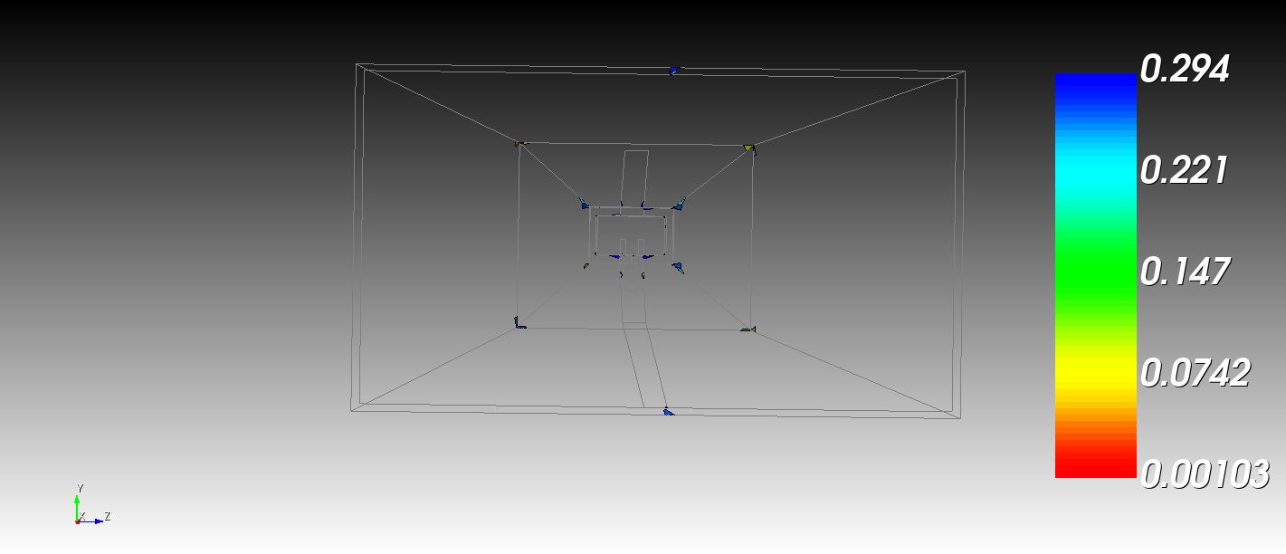
My CAD Model:
- Is sending by Mail (can’t it upload)
My material library:
from nsem import *
ml = MaterialLibrary()
ml.add_material(Material(‘RO3003’,‘green’,MaterialProperty(‘constant’,real=3.0,imag=-3.0*0.001),MaterialProperty(‘constant’,real=1.0,imag=0.0)))
ml.add_material(Material(‘Teflon’,‘yellow’,MaterialProperty(‘constant’,real=2.1,imag=-2.1*0.0002),MaterialProperty(‘constant’,real=1.0,imag=0.0)))
ml.add_material(Material(‘air’,‘blue’, MaterialProperty(‘constant’,real=1.0,imag=0.0),MaterialProperty(‘constant’,real=1.0,imag=0.0)))
ml.add_material(Material(‘duroid5880’, ‘green’, MaterialProperty(‘constant’, real = 2.2, imag = -2.2*0.0009), MaterialProperty(‘constant’, real = 1.0, imag = 0.0)))
ml.add_material(Material(‘dielectric’,‘red’, MaterialProperty(‘constant’,real=4.0,imag=-0.2),MaterialProperty(‘constant’,real=1.0,imag=0.0)))
ml.add_material(Material(‘fake’,‘red’, MaterialProperty(‘constant’,real=10.0,imag=-0.0),MaterialProperty(‘constant’,real=1.0,imag=0.0)))
ml.save(r’E:\Michael\Nullspace_workspace\Material\materials’)
My .jou
reset
reset aprepro
#{vs_w = 2}
#{freq = 16e9}
#{co = 3e8}
#{lambda = (co/freq)*1000}
#{lambda_length = lambda}
#{lambda_length = 2}
import acis “E:/Michael/Nullspace_workspace/Exapels/NSEM_Online_Tutorial_Patch_antenna/Antenne_neu v12.sat” nofreesurfaces heal attributes_on separate_bodies
volume 1 rename “Back_A”
volume 2 rename “Frame”
volume 3 rename “Taper_1”
volume 5 rename “Coax_di”
volume 4 rename “Pin”
volume 6 rename “Taper_2”
create surface rectangle width {vs_w} zplane
volume 7 rename “feed”
move volume feed x {-21.5} y {-100-vs_w/2} z {0} include_merged
split surface 87 direction curve 207
project surface 67 onto surface 72 imprint
split periodic volume 4
imprint tolerant volume all tolerance 10e-3
merge volume all
##split curve 206 at vertex 131 157 ## split surface of Pin same like the oposit side
set duplicate block elements off
block 1 add surface all
block all element type quad9
nsem load material library “E:\Michael\Nullspace_workspace\Material\materials.h5”
nsem assign volume {Id(“Back_A”)} material ‘PEC’
nsem assign volume {Id(“Frame”)} material ‘PEC’
nsem assign volume {Id(“Pin”)} material ‘PEC’
nsem assign volume {Id(“Taper_1”)} material ‘PEC’
nsem assign volume {Id(“Taper_2”)} material ‘PEC’
nsem assign volume Coax_di material ‘Teflon’
nsem assign surface 123 125 128 129 91 131 132 material ‘PEC’ ## surface coax_di/freespace; surface top inside antenna
nsem voltage source ‘port1’ pos surface 88 neg surface 89 impedance 50
surface all scheme pave
curve 209 211 215 interval 1
curve 209 211 215 scheme equal
surface in volume feed size
mesh surface in volume feed
meshing small surfaces in Volume Back_A with smaler size couse its necessary
surface 1 18 19 20 27 2 3 4 15 16 17 21 22 23 24 25 26 size {0.5}
mesh surface 1 18 19 20 27 2 3 4 15 16 17 21 22 23 24 25 26
surface not is_meshed in volume Pin size {lambda_length/3}
mesh surface not is_meshed in volume Pin
surface in volume Taper_1 size {lambda_length/3}
mesh surface in volume Taper_1
surface in volume Taper_2 size {lambda_length/3}
mesh surface in volume Taper_2
surface in volume Coax_di size {lambda_length/3}
mesh surface in volume Coax_di
surface not is_meshed size {lambda_length*2}
mesh surface not is_meshed
My simulation .py
import numpy as np
from nsem.material_library import *
from nsem.config import *
from nsem.report import *
Include materials for the model to simulate it
ml = MaterialLibrary()
ml.load(r’E:\Michael\Nullspace_workspace\Material\materials’)
#Config the model
mesh_name = ‘Antenna mesh new.cub5’ #Name of the cub5 / Meshfile %Auf dauer durch suche nach ‘Mesh’ ersetzen
config_name = ‘_HF906_rcs_surface_C_V_10’ #Name of the h5 data
freq = 1 #Frequency for simulation range vec. or scal.
thInc = np.linspace(0,180.0,10) #Theata angle of excitation also possible as vec. than you have more excitations
phInc = [0.0, 45.0, 90.0 ] #Phi angle of excitation also possible as vec. than you have more excitations
model = Configuration(‘Sim’+f’{config_name}')
model.set_cub5_filename(mesh_name)
model.set_order(1) #Basicfunction order (1-3)
model.set_solve_type(‘dense’) #Set solver propertys, default is dense for big models use compress
model.set_frequencies(freq)
model.set_model_scale(0.001)
model.save(ml) #Save the config to h5 file, here also the material parameter
#Report
#Report can also be seperated from the sim,
#so you don’t have to simulate every time ne if
#you want change the report data
#Config the report
report = Report(‘Rep’+f’{config_name}', model)
thObs = np.linspace(0,180,721)
phObs = 0.0
#Define which results you want to see
report.request_far_fields_grid(thObs, phObs) #Define the observation angle of the far field, relevant for RCS Plotts, they show the reflection of a divice
report.request_y_parameters()
report.request_paraview(type=‘xmf’,num_samples=3)
report.request_surface_currents(type=‘centroid’, request_abs=True, request_real=False, request_imag=False)
report.save()
model.run()
report.run()
My post .py
import matplotlib.pyplot as plt
from nsem.postprocessing import *
config_name = ‘_HF906_rcs_surface_C_V_10’
post = PostProcess(r’E:\Michael\Nullspace_workspace\HF906_Antenna’+‘\’+‘Rep’+f’{config_name}')
thInc = post.get_inc_theta()
thObs = post.get_obs_theta()
phInc = post.get_inc_phi()
phObs = post.get_obs_phi()
RCSm = post.get_rcs(‘spherical’, ‘dB’)
freq = post.get_frequencies()
d_sphere = 8*speed_of_light/10e9
lam_over_freq = speed_of_light/(freq*1e9)
s = post.get_s_parameters()
ReturnLoss = dB20(np.squeeze(s[0,0,:]))
z = post.get_input_impedance()
z_real = np.real(np.squeeze(z[0,:]))
z_imag = np.imag(np.squeeze(z[0,:]))
z = np.squeeze([z[0,:]])
g = post.get_gain(‘spherical’)
g_boresight = np.squeeze(g[0, 0, 0, :, 0])
fig = plt.figure()
ax = fig.add_subplot(1,1,1)
ax.plot(freq, dB20(np.squeeze(s[0,0,:])), color=‘b’, linestyle=‘-’, linewidth=2.0)
ax.plot(freq, dB20(np.squeeze(s[1,0,:])), color=‘r’, linestyle=‘-’, linewidth=2.0)
Combine feeds for RHCP
weights = [1j, 1]
active_s = post.get_active_s_parameters(weights)
ax.plot(freq, dB20(active_s[0,:]), color=‘k’, linestyle=‘-’, linewidth=2.0)
ax.set_title(r’$S$-Parameters’)
ax.set_ylabel(r’$S_{mn}$ (dB)')
ax.set_xlabel(‘Frequency (GHz)’)
ax.grid(True)
ax.legend([r’$S_{11}$‘, r’$S_{21}$‘, r’Active $S_{1}$’])
Calculate and plot boresight directivity in RHCP/LHCP
th = post.get_obs_theta()
ph = post.get_obs_phi()
d = post.get_directivity(‘circular’, weights)
fig = plt.figure()
ax = fig.add_subplot(1,1,1)
thIdx, thVal = post.get_nearest(th, 90.0)
d_boresight = np.squeeze(d[0, thIdx, 0, :, 0])
ax.plot(freq, d_boresight, f’b-', linewidth=2.0)
d_boresight = np.squeeze(d[0, thIdx, 0, :, 1])
ax.plot(freq, d_boresight, f’r-', linewidth=2.0)
g_boresight = np.squeeze(g[0, thIdx, 0, :, 0])
ax.plot(freq, g_boresight, f’b–', linewidth=2.0)
g_boresight = np.squeeze(g[0, thIdx, 1, :, 1])
ax.plot(freq, g_boresight, f’r–', linewidth=2.0)
ax.set_title(r’Boresight Gain’)
ax.set_ylabel(r’Gain (dB)')
ax.set_xlabel(r’Frequency (GHz)')
ax.grid(True)
ax.legend([r’$D_{\mathrm{RHCP}}$‘, r’$D_{\mathrm{LHCP}}$', \
r’$G_{\mathrm{RHCP}}$‘, r’$G_{\mathrm{LHCP}}$'])
Plot theta- and phi-cuts
fqIdx, fqVal = post.get_nearest(freq, 20.0)
phIdx, phVal = post.get_nearest(ph, 0.0)
fig = plt.figure()
ax = fig.add_subplot(1,1,1)
ax.plot(th, g[phIdx,:,0,fqIdx,0], ‘b-’, linewidth=2.0)
ax.plot(th, g[phIdx,:,0,fqIdx,1], ‘r-’, linewidth=2.0)
ax.set_title(r’Gain Pattern : $\phi = 0^{\circ}$')
ax.set_ylabel(‘Gain (dB)’)
ax.set_xlabel(r’$\theta$ (deg)')
ax.grid(True)
ax.legend([‘RHCP’, ‘LHCP’])
fig = plt.figure()
ax = fig.add_subplot(1,1,1)
ax.plot(ph, g[:,thIdx,0,fqIdx,0], ‘b-’, linewidth=2.0)
ax.plot(ph, g[:,thIdx,0,fqIdx,1], ‘r-’, linewidth=2.0)
ax.set_title(r’Gain Pattern : $\theta = 90^{\circ}$')
ax.set_ylabel(‘Gain (dB)’)
ax.set_xlabel(r’$\phi$ (deg)')
ax.grid(True)
ax.legend([‘RHCP’, ‘LHCP’])
Export 3D RHCP and LCHP gain patterns for Paraview
post.generate_3D_fields_paraview(g, ‘g_rhcp.vtk’, fqIdx, 0, polarization = 0, scalemin = -10, scalemax = 10)
post.generate_3D_fields_paraview(g, ‘g_lhcp.vtk’, fqIdx, 0, polarization = 1, scalemin = -10, scalemax = 10)
The postscript is more or less copied from your patch antenna tutorial, as well as the simulation program. I try to do it as simple as possible.
The mesh status:
Summary
Face quality, 92639 elements:
Function Name Average Std Dev Minimum (id) Maximum (id)
Shape 9.865e-01 4.859e-02 1.026e-03 (25842) 1.000e+00 (74428)
And here is the error:
PS E:\Michael\Nullspace_workspace\Exapels\Sphere_RCS_Surface_C> & “C:/Program Files/Nullspace EM 2023 R3/Nullspace-Python/python.exe” e:/Michael/Nullspace_workspace/HF906_Antenna/Post_HF906.py
Traceback (most recent call last):
File “e:\Michael\Nullspace_workspace\HF906_Antenna\Post_HF906.py”, line 16, in
s = post.get_s_parameters()
File “C:\Program Files\Nullspace EM 2023 R3\Nullspace-Python\lib\site-packages\nsem\postprocessing.py”, line 794, in get_s_parameters
sol = linalg.solve((I+zYz),(I-zYz))
File “C:\Program Files\Nullspace EM 2023 R3\Nullspace-Python\lib\site-packages\scipy\linalg_basic.py”, line 143, in solve
ce-Python\lib\site-packages\scipy_lib_util.py", line 252, in _asarray_validated
ce-Python\lib\site-packages\scipy_lib_util.py", line 252, in _asarray_validated
ce-Python\lib\site-packages\scipy_lib_util.py", line 252, in _asarray_validated
a = toarray(a)
File “C:\Program Files\Nullspace EM 2023 R3\Nullspace-Python\lib\site-packages\numpy\lib\function_base.py”, line 628, in asarray_chkfinite
raise ValueError(
ValueError: array must not contain infs or NaNs
PS E:\Michael\Nullspace_workspace\Exapels\Sphere_RCS_Surface_C> & “C:/Program Files/Nullspace EM 2023 R3/Nullspace-Python/python.exe” e:/Michael/Nullspace_workspace/HF906_Antenna/Post_HF906_clean.py
Traceback (most recent call last):
File “e:\Michael\Nullspace_workspace\HF906_Antenna\Post_HF906_clean.py”, line 18, in
s = post.get_s_parameters()
File “C:\Program Files\Nullspace EM 2023 R3\Nullspace-Python\lib\site-packages\nsem\postprocessing.py”, line 794, in get_s_parameters
sol = linalg.solve((I+zYz),(I-zYz))
File “C:\Program Files\Nullspace EM 2023 R3\Nullspace-Python\lib\site-packages\scipy\linalg_basic.py”, line 143, in solve
a1 = atleast_2d(_asarray_validated(a, check_finite=check_finite))
File “C:\Program Files\Nullspace EM 2023 R3\Nullspace-Python\lib\site-packages\scipy_lib_util.py”, line 252, in _asarray_validated
a = toarray(a)
File “C:\Program Files\Nullspace EM 2023 R3\Nullspace-Python\lib\site-packages\numpy\lib\function_base.py”, line 628, in asarray_chkfinite
raise ValueError(
ValueError: array must not contain infs or NaNs
For postprocessing, there isn’t any data for S-Parameter or for Impedance. The sim runs up to 3 hours which is realistic for a simulation with the amount of Basisfunctions and Meshcells.
Have you any idea what could help or I can try?